

The Physical Reality of Wind Tunnel Testing (Why Virtual Simulators Precede the Test Section)
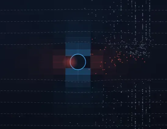
In any experimental aerodynamics lab, the fastest way to waste test section hours is mounting a scale model without first running flow diagnostics. When you bolt a 3D-printed wing or vehicle model to a strain-gauge balance inside a subsonic test section, you are measuring a coupled system where the model's boundary layer interacts with solid tunnel walls, nozzle boundary layer displacement, pitot calibration drift, and barometric density variations.
A dedicated aerodynamic wind tunnel simulator allows you to verify boundary layer attachment, anticipate adverse pressure gradients, and predict the onset of stall before expending compressor power. Using this online wind tunnel simulator, you can solve discretized Navier-Stokes transport equations across 2D geometries to visualize stagnation points, suction peaks, and wake vortex shedding in real time. Accessing a high-fidelity wind tunnel simulator free in your browser bridges theoretical fluid mechanics with physical wind tunnel data reduction.
Boundary Layer Physics: Pressure Gradients, Suction Peaks, and Stall
Aerodynamic forces originate from only two physical mechanisms acting on a body's wetted surface: the normal distribution of static pressure (p) and the tangential distribution of wall shear stress (τw).
When fluid approaches an airfoil's leading edge, it decelerates to a complete stop at the stagnation point, where the pressure coefficient reaches exactly Cp = +1.0. As flow curves over the upper convex suction surface, it accelerates past the freestream velocity, causing static pressure to plummet (Cp < 0). This creates the pressure differential that generates lift.
However, past the suction peak, the flow must travel toward the trailing edge where pressure returns toward atmospheric levels. This region of rising pressure is an adverse pressure gradient (dp/dx > 0). Fluid inside the viscous boundary layer has already lost kinetic energy due to wall shear friction. If the adverse pressure gradient is too steep — such as when the angle of attack (α) exceeds 14° — the near-wall flow runs out of momentum, stagnates, and reverses direction:
- Laminar Separation Bubble (LSB): At low Reynolds numbers (Re < 5 × 10⁵), laminar boundary layers detach easily under mild adverse gradients, transition to turbulence in mid-air, and may reattach downstream, creating a drag bubble.
- Trailing-Edge Stall: On moderately thick airfoils (like the NACA 4412), turbulent separation begins at the trailing edge and creeps forward as α increases, causing a progressive, gentle loss of lift.
- Leading-Edge Stall: On thin sections or sharp edges, separation occurs abruptly at the nose, causing catastrophic lift collapse and sudden pitching moments.
The Wind Tunnel Blockage Effect: Why Uncorrected Data Lies
One of the most persistent traps in aerodynamic testing is testing a model that occupies too large a fraction of the test section. In free flight, air can deflect infinitely around an aircraft. Inside a closed wind tunnel, the solid ceiling and floor prevent streamtube expansion.
The model volume constricts the passage area, forcing the surrounding air to speed up. This phenomenon consists of solid blockage (εsb) from the physical model volume and wake blockage (εwb) from the slower, low-pressure wake behind the body:
Because the local velocity past the model is higher than the upstream freestream velocity measured by the reference pitot-static tube, uncorrected test data produces dynamic pressures that are too low and force coefficients that are artificially high. Using the standard Barlow-Rae-Pope formulation, we correct the raw test numbers:
As a golden rule of wind tunnel testing, keep the model's frontal area below 5% of the test section cross-sectional area. Beyond 7%–10% blockage, linear correction models break down because the pressure gradient along the test section creates an artificial buoyancy force that distorts drag readings.
Dynamic Similarity and Sutherland's Viscosity Law
Testing a 1:10 scale car model at highway speed (30 m/s) does not reproduce highway aerodynamics. Dynamic similarity requires matching the non-dimensional Reynolds number, not the physical velocity:
Because the model length (L) is 10 times smaller, matching Re at ambient temperature would require a tunnel speed of 300 m/s (nearly Mach 0.9). At that speed, air is no longer incompressible; compressibility shocks form, invalidating the test. If your research involves transonic or supersonic Mach regimes, verify shock wave angles with our Compressible Flow Simulator.
Furthermore, air dynamic viscosity (μ) is strongly temperature-dependent. On a cold morning in an unheated tunnel (5°C vs. 30°C in summer), viscosity changes by more than 6% according to Sutherland's formula (Sμ = 110.4 K, T0 = 273.15 K, μ0 = 1.716 × 10⁻⁵ Pa·s). Always log ambient temperature and barometric pressure before zeroing your transducers.
Aerodynamic Profile & Flow Regime Comparison Matrix
The table below compiles aerodynamic benchmarks across standard 2D and axisymmetric geometries operating in the subcritical to supercritical Reynolds regimes:
| Test Profile | Laminar CD | Turbulent CD | Separation Angle (θsep) | Dominant Drag Form | Stall αstall | Strouhal (St) |
|---|---|---|---|---|---|---|
| NACA 0012 Airfoil | 0.008 – 0.012 | 0.006 – 0.009 | Trailing edge (α < 12°) | Skin Friction (85%) | 14.5° – 16.0° | N/A (Attached) |
| NACA 4412 Cambered | 0.009 – 0.014 | 0.007 – 0.010 | Trailing edge (α < 14°) | Skin Friction (80%) | 15.5° – 17.0° | N/A (Attached) |
| Circular Cylinder | 1.15 – 1.25 | 0.30 – 0.40 | 82° (Lam) / 120° (Turb) | Form Pressure (95%) | N/A (Bluff) | 0.20 – 0.21 |
| Smooth Sphere | 0.47 – 0.50 | 0.15 – 0.20 | 84° (Lam) / 125° (Turb) | Form Pressure (92%) | N/A (Bluff) | 0.18 – 0.22 |
| Flat Plate (Normal) | 1.95 – 2.05 | 1.95 – 2.05 | 0° (Sharp Edge) | Form Pressure (100%) | N/A (Bluff) | 0.14 – 0.16 |
| Streamlined Teardrop | 0.045 – 0.060 | 0.035 – 0.045 | Aft Cusp (95% Chord) | Skin Friction (75%) | N/A | N/A (Attached) |
Worked Lab Calculation: NACA 4412 Wing in Subsonic Tunnel
Let us walk through a complete, non-idealized wind tunnel data reduction for a cambered wing model tested in a closed test section:
- Wing Model: NACA 4412 profile, chord c = 0.180 m, span b = 0.540 m, max thickness t/c = 12%
- Test Section: Square cross-section 0.60 m × 0.60 m (Area Ctunnel = 0.360 m2)
- Atmospheric Conditions: Temperature T = 18.5°C (291.65 K), Ambient pressure Pamb = 100.8 kPa
- Measured Airspeed: Pitot-static reading U∞ = 28.4 m/s
- Raw Balance Readings at α = 7.5°: Lift force Lmeas = 43.8 N, Drag force Dmeas = 3.65 N
Step 1: Atmospheric Density and Viscosity
Using the ideal gas equation of state (Rspecific = 287.05 J/(kg·K)) and Sutherland's law:
Step 2: Chord Reynolds Number & Uncorrected Dynamic Pressure
Step 3: Uncorrected Aerodynamic Coefficients
Planform area S = c · b = 0.180 · 0.540 = 0.0972 m2, Aspect Ratio AR = b2 / S = 0.5402 / 0.0972 = 3.0:
Step 4: Blockage Corrections (Barlow-Pope Model)
Model frontal area Sfrontal ≈ c · t · b + S sin(7.5°) = (0.180 · 0.0216 · 0.540) + (0.0972 · 0.1305) ≈ 0.00210 + 0.01269 = 0.01479 m2. With solid blockage εsb = 0.0185:
Step 5: Corrected Performance Coefficients
Instructor's Takeaway: Without blockage correction, lift would have been overstated by 4.0% (0.9280 vs 0.8923) and drag by 4.0% (0.0773 vs 0.0744). Using a wind tunnel simulator online allows engineers to verify these calibration shifts before running physical tests. If you need a wind tunnel simulator online free of software installation for rotational blade design, explore how local twist changes relative inflow in our Wind Turbine Simulator, or compute internal pipe friction losses in the Hydraulic Flow Calculator.
Four Hard-Earned Rules from 15 Years in the Wind Tunnel Lab
- Respect the 5% Blockage Barrier: Never size a model whose frontal area exceeds 5% of the test section nozzle area. If forced to test at 7%–8% blockage, apply both solid and wake blockage corrections immediately. Beyond 10%, wall-induced streamline curvature renders data meaningless.
- Trip Your Boundary Layers on Scale Models: Testing airfoils at low chord Reynolds numbers (Re < 3 × 10⁵) without turbulator tape causes massive laminar separation bubbles that do not exist at full scale. Apply 0.1 mm carborundum grit or zigzag trip tape at 5% chord on the suction surface to force turbulent transition.
- Log Daily Temperature and Barometer Readings: Never assume standard sea-level air (ρ = 1.225 kg/m3). A weather low-pressure system combined with summer heat can easily drop air density to 1.15 kg/m3 — a 6% error in force measurements if uncorrected.
- Never Confuse 2D Profile Drag with 3D Wing Drag: A 2D airfoil in a virtual simulator or endplate tunnel produces only profile drag (Cd = Cd,friction + Cd,form). A real 3D finite wing incurs induced drag (CDi = CL2 / (π e AR)) from wingtip downwash, which often accounts for 40% to 70% of total cruise drag.
Frequently Asked Questions (FAQ)
What causes aerodynamic stall on an airfoil?
Stall occurs when the angle of attack exceeds the critical limit (typically 12° to 16°). The severe adverse pressure gradient (dp/dx > 0) on the upper suction surface decelerates near-wall fluid until shear stress drops to zero and flow reverses, detaching the boundary layer and destroying lift.
Why do scale models in wind tunnels need blockage corrections?
In closed test sections, the model and wake constrict the passage area, accelerating surrounding airflow. This increases local dynamic pressure above upstream reference levels. Without Pope/Barlow corrections, measured lift and drag coefficients are overstated by 2% to 15%.
How does dynamic similarity differ from matching velocity?
Dynamic similarity requires matching the Reynolds number (Re = ρ U L / μ), not velocity. Because scale models have smaller characteristic lengths, matching Re requires higher velocity, pressurized air, or cryogenic cooling to reduce kinematic viscosity.
What is the difference between 2D section drag and 3D wing drag?
A 2D airfoil has infinite span and produces only profile drag (skin friction and form drag). A 3D finite wing creates wingtip vortices due to spanwise pressure leakage, generating downwash that tilts the lift vector backward and adds induced drag (Cdi = Cl2 / (π e AR)).
What causes the drag crisis on spheres and cylinders?
Near Re ≈ 3 × 10⁵, the boundary layer transitions from laminar to turbulent before separating. Turbulent fluid has higher momentum, delaying separation from 82° to 120°, shrinking the wake and causing Cd to collapse from 0.47 to 0.18.